This is the third of four articles on tomography (also read the first one, the second one, and the fourth one).
At the end of the second article, I left you with a very blurry reconstruction of the scanned object. Indeed, naive backprojection is not sufficient to create high-quality reconstructions. Why is that so?
Intuitively, a simple backprojection cannot be expected to create a perfect reconstruction, since the contribution of all smeared-back projections is positive everywhere. This means that even pixels outside of the object can get a positive value. Clearly, something is wrong here. Leaving out the details (I should write a separate article on the Fourier transform to really explain what is going on), the problem is that the information about the object is not homogeneous in frequency space (i.e., after taking the Fourier transform). It might seem strange to think about an image as containing different (spatial) frequencies, but compare this with the frequency contents of sound: The human ear directly perceives frequency information in sounds, and the actual waveform doesn’t mean much to us. For images, this is the other way around, since the human eye detects the brightness of an image, and not the frequency contents. But the frequency contents is there, and, just as for sound, you can go back and forth between the two representations without losing information.
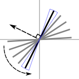
 Fourier slice theorem.
Now, due to the way that the object is recorded by the different projections, there is more information about the low frequencies than about the high frequencies. Mathematically, this follows from the Fourier slice theorem, which (loosely) states that the Fourier transform of each projection provides information, in frequency space, on a line through the origin that is perpendicular to the direction of that projection. In the figure to the right, the black line represents the frequency information that is provided by the projection in the direction of the straight arrow. As each line passes through the origin, there is more information in the vicinity of the origin (where the low frequency information is) than near the borders (where the high frequency information is). And, since high frequencies contain information about small details, less high frequency information means that the reconstruction is going to be blurry. Note that this also shows directly that each projection provides information about the object that is almost entirely independent, since the information in frequency space only overlaps in the center. This independence might not be intuitively clear from the projections in object space, since neighboring projections are, after all, “pretty close together”.
Filtered Backprojection
To compensate for the relative lack of high frequencies, low frequencies are attenuated in the projections before backprojection. This is the so-called filtered backprojection. The amount of attenuation follows from the geometry of the frequency space information. Each line in the above figure is taken to represent a wedge (indicated by the blue dotted line). As there is not enough high frequency information to “fill” the wedge at higher frequencies (away from the origin), the data is multiplied with a correction factor. This factor linearly increases from zero in the origin to one for the highest frequencies. This is, of course, an approximation, since the missing high frequency data doesn’t magically appear in this way, but one that can be made as good as needed by increasing the number of projections.
Reconstructions created with filtered backprojection, together with the original objects, are shown below. As you can see, the reconstructed slices (rightmost two images) are now very close to the original objects (leftmost two images). Variations of the filtered backprojection algorithm are widely used in medical CT (CAT) scanners.
 Reconstructions of box with ball
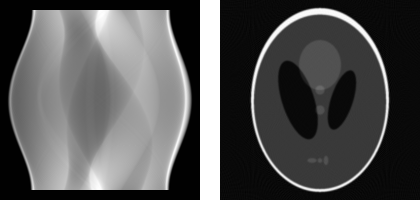
As an example of a somewhat more complicated object, and since I’ve already told you that the Shepp-Logan phantom is used often as a test image in CT, I show its sinogram (180 projections) and reconstruction below. As you can see, for an object of this size (200 by 200 pixels), a reconstruction from 180 projections is quite accurate.
 Shepp-Logan sinogram (left). Shepp-Logan reconstruction (right)
The next article explains how algebraic techniques can be used for tomographic reconstruction. This is where most research (including my own) is situated nowadays.
Add new comment