Spectral Reversal to Create a High-Pass Filter

This article presents spectral reversal, a technique to turn a low-pass filter into a high-pass filter. Spectral reversal is an alternative for spectral inversion, as described in How to Create a Simple High-Pass Filter.

The windowed-sinc filter that is described in this article is an example of a Finite Impulse Response (FIR) filter.

Spectral Reversal

Starting from the cutoff frequency \(f_c\) and the transition bandwidth (or roll-off) \(b\), first create a low-pass filter as described in How to Create a Simple Low-Pass Filter. The normalized low-pass filter from that article, again for \(f_c=0.1\) and \(b=0.08\), is shown as the left image in Figure 1.

The spectral reversal of a filter \(h[n]\) is computed by changing the sign of every other value in \(h[n]\), i.e., by multiplying \(h[n]\) with the sequence \(1,-1,1,-1,\ldots\) Hence, the coefficients of the new filter can be written elegantly as \((-1)^nh[n]\).

This produces the filter shown as the right image in Figure 1.

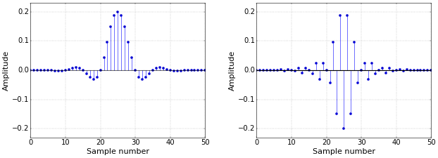Figure 1. Low-pass (left) and high-pass (right) filters.

The frequency response of the high-pass filter is then as shown in Figure 2.

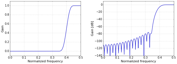Figure 2. Frequency response on a linear (left) and logarithmic (right) scale.

This frequency response is a “left-right flipped” version of the frequency response of the low-pass filter. In contrast, the spectral inversion filter from How to Create a Simple High-Pass Filter was an “upside down” version of the original low-pass filter.

Why Does Spectral Reversal Work?

The spectral reversal technique is based on the so-called shift theorem of the Fourier transform. Formulated for the discrete case, the shift theorem says that, for a Fourier transform pair \(x[n]\longleftrightarrow X[k]\), a shift by \(s\) samples in the frequency domain is equivalent with multiplying by a complex exponential in the time domain, as

\[x[n]e^{i2\pi ns/N}\longleftrightarrow X[k-s].\]

In general, the result of doing this will be complex. This is not a problem, but let’s investigate in which circumstances the result is not complex. This is may be easiest to see with the complex exponential rewritten using Euler’s Identity,

\[e^{i2\pi ns/N}=\cos(2\pi ns/N)+i\sin(2\pi ns/N).\]

This expression is real if the sine term is zero, which is the case if the angle is zero or \(\pi\).

We get this result if we shift by \(s=N/2\) samples, because then the angles become \(2\pi ns/N=n\pi\). Of course, in that case the complete expression becomes \(\cos(n\pi)\), which is exactly the sequence \(1,-1,1,-1,\ldots\)

To see why shifting by \(N/2\) samples turns a low-pass filter into a high-pass filter, we first have to look at a double sided spectrum of the original low-pass filter (Figure 3).

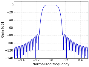Figure 3.

Normally, the negative frequencies are not very interesting for the real filters that we have been working with, since they are simply the mirror image of the positive frequencies. However, shifting the filter over a number of samples results in a complex filter, for which the frequency response is generally no longer symmetrical around zero. For example, Figure 4 shows the response of the filter with \(h[n]\) shifted by 10 samples through multiplying by the complex exponential given above. The filter has changed into a (complex) band-pass filter!

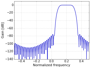Figure 4.

It just happens that a shift by \(N/2\) samples shifts this band-pass filter around the (normalized) frequency of 0.5 (half of the sampling frequency in general). This is shown in Figure 5, for a shift of 25.5 samples, since the length of \(h[n]\) is 51.

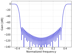Figure 5.

And this just happens to be a real frequency response again, since it is symmetrical around zero. If you look at the part between zero and 0.5, it is exactly the same as the plot in Figure 2. Hence, spectral reversal produces a high-pass filter if you start from a low-pass one.

Python Code

In Python, spectral reversal can be implemented concisely through

h *= (-1) ** np.arange(N)

I am aware that this is probably not the most efficient implementation, but efficiency is not really important here, and if that is the case, I’m normally in favor of following the mathematics as closely as possible in the implementation. There is a complete script in How to Create a Simple High-Pass Filter, where you can then simply replace the two last lines with the one line given above.