Variations on the Moving Average

The moving-average filter is more or less perfect for smoothing data in the presence of noise, if the useful information in your data is completely in the time domain. In that case, you don’t care about its rather poor performance in the frequency domain. Figure 1 shows the impulse, step, and frequency responses of the basic moving-average filter (with three extra samples on both sides that are not part of the impulse and step responses, for clarity).

Figure 1. Impulse (left), step (middle), and frequency (right) responses for the moving-average.

Sometimes, however, you have to work with data for which both domains are important. For those cases, there are “weighted” versions of the moving average that are more or less equivalent in the time domain, but that have much better performance in the frequency domain.

Repeated Moving Average

The first thing that you can do to improve the frequency response of the moving-average is to apply it several times. After two repetitions, this amounts to a triangular weighting of the coefficients (Figure 2). Since applying the same filter twice doubles its effect, the first side lobe of the frequency response is only half as high as the one of Figure 1. The reason for the triangular shape is that the moving average is a convolution with a rectangular pulse. Applying it twice causes a convolution of this rectangular pulse with itself, resulting in a triangular window for the combined filter. Note that I’ve taken the same filter length in Figure 2 as in Figure 1, thereby shifting the first zero of the frequency response. A true convolution of the original rectangular filter would have resulted in a longer filter and would have kept the zeros in exactly the same place, of course.

Figure 2. Impulse (left), step (middle), and frequency (right) responses for the triangular window.

If the moving-average filter is repeated multiple times, its coefficients converge to a Gaussian window (Figure 3) because of the central limit theorem. Of course, an actual Gaussian extends infinitely in both directions, so there is no other option than to cut it of at some point (or perhaps multiply it by a second window). Additionally, the standard deviation of the Gaussian has to be chosen. For this illustration (and for the implementation of the Filter Designer), I have adopted the default settings of MATLAB.

Figure 3. Impulse (left), step (middle) and frequency (right) responses for the Gaussian window.

In practice, you might want to simply repeatedly apply the moving average instead of applying a Gaussian window. When implemented recursively, the moving average is very efficient, while the Gaussian window must be implemented through convolution.

Blackman Window

Another possibility is to pick one of the classical window functions that are used for windowed-sinc filters, and use that as a filter kernel (see the excellent Wikipedia page on window functions). As an example, I’ve picked the Blackman window (Figure 4). This improves the stop-band attenuation even further, while still showing a smooth time domain response without any ringing or overshoot.

Figure 4. Impulse (left) and frequency (right) responses for the Blackman window.

In conclusion, if you need to smooth data but need a better frequency performance than the basic moving average has to offer, several alternatives are available.

Filter Design Tool

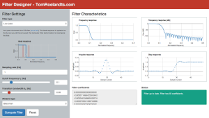
This article is complemented with a Filter Design tool. Experiment with the different window functions and the length of the filter, and see the effect on the frequency response. Try it now!

Filter designer.