This article shows how to plot the frequency response of the filters that I describe in my articles on filter design. Plotting this kind of frequency response should not be confused with the spectral density estimation of measured signals, which can be (much) more involved. For the specific case of a filter, however, the frequency response tells you exactly how each frequency is altered. The example code is in Python, as usual, but the methodology is applicable for any programming language or plotting tool.
Time and Frequency Representation
The main operation that will get you from the time domain to the frequency domain is the Discrete Fourier Transform (DFT). In practice, you’ll typically use the Fast Fourier Transform (FFT) , which is an efficient algorithm for computing the DFT.
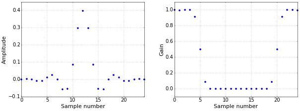
A crucially important point is that simply computing the FFT of the filter is not enough. As an example, Figure 1 shows a low-pass filter, as presented in How to Create a Simple Low-Pass Filter, both in the time domain (left) and in the frequency domain (right).
 Figure 1. Time domain (left) and frequency domain (right) representation of a filter.
The dots in the frequency domain plot are exactly the result of the FFT, but, by themselves, they don’t give you a clear picture of the true frequency response. There are at least three reasons for this:
- The frequency response of a discrete-time (or digital) filter is continuous, even though the Fourier transform is a finite number of points.
- The response that is plotted is typically from 0 Hz to half of the sampling rate. However, the actual result of the FFT contains a mirror of this in its second half (in the more general case of filters with complex coefficients this is no longer true, but I’ll keep that for a future article).
- The plot has a linear scale, while frequency plots mostly have a logarithmic scale (in dB).
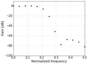
As a first step towards the typical frequency response plots that you are probably more familiar with, Figure 2 shows only the first half of the FFT, in dB. I have an article on the normalized frequency that is used on the X axis, if you are curious.
 Figure 2. Frequency response of filter in dB.
Continuous Frequency Response
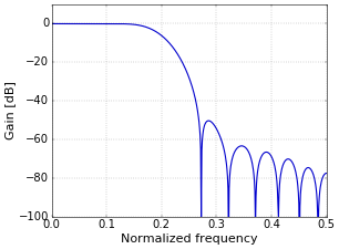
The dots in Figure 2 are samples of the complete frequency response. However, the actual frequency response of the filter is, of course, continuous, since it has an exactly defined effect on every frequency that you put through the filter. To show the continuous frequency response of the filter, some more work is needed. The way to do this is to “pad with zeros”. You increase the length of the time signal, typically to a power of two such as 1024 (the power of two is only for the FFT algorithm). The reason that you are allowed to do this, is that adding zeros does not change the filter, since the zeros have no effect. However, the result of the FFT of this longer signal, still only samples of the true response, will be smooth when plotted in a graph. The result of padding with zeros to a length of 1024 samples is shown in Figure 3.
 Figure 3. Frequency response of padded filter.
The plot of Figure 3 is exactly how I normally present frequency response plots. Python code that creates this plot follows in the next section.
Python Code
from __future__ import division

import numpy as np
import matplotlib.pyplot as plt

fc = 0.2  # Cutoff frequency as a fraction of the sampling rate (in (0, 0.5)).
N = 25    # Number of coefficients.
L = 1024  # Length of frequency response.

# Compute sinc filter with Hamming window.
n = np.arange(N)
h = np.sinc(2 * fc * (n - (N - 1) / 2)) * np.hamming(N)
h /= np.sum(h)

# Pad filter with zeros.
h_padded = np.zeros(L)
h_padded[0 : N] = h

# Compute frequency response; only keep first half.
H = np.abs(np.fft.fft(h_padded))[0 : L // 2 + 1]

# Plot frequency response (in dB).
plt.figure()
plt.plot(np.linspace(0, 0.5, len(H)), 20 * np.log10(H))
plt.xlabel('Normalized frequency')
plt.ylabel('Gain [dB]')
plt.ylim([-100, 10])
plt.grid()
plt.show()
Tom,
With the latest Python 3 you need to make a minor tweak to this line:
H = np.abs(np.fft.fft(h_padded))[0 : L / 2 + 1]
and update it to be
H = np.abs(np.fft.fft(h_padded))[0 : L // 2 + 1]
Otherwise Python will complain about indexing with a non-integer value.
Thanks for all the great writeups.
Thanks for the hint! I've adapted the code.
It would be interesting to have a python function that has the functionality of the function freqz() in Matlab/octave. It provides the frequency response for a given set of coefficients (works for fir and iir filters)
There is a version of freqz in sicpy.signal.
Please can you explain how can we use it for a sobel filter ?
Ps I just stumbled upon your nice blog site!
It reminds me of www.earlevel.com, a site that I check regularly for DSP audio stuff.
The FFT calculation can be expressed more simply by using numpy's real fft as follows:
H = np.abs(np.fft.rfft(h_padded))
Chris
Even simpler is:
H = abs(np.fft.rfft(h, n=L))Add new comment