The moving average is often used for smoothing data in the presence of noise. The simple moving average is not always recognized as the Finite Impulse Response (FIR) filter that it is, while it is actually one of the most common filters in signal processing. Treating it as a filter allows comparing it with, for example, windowed-sinc filters (see the articles on low-pass, high-pass, and band-pass and band-reject filters for examples of those). The major difference with those filters is that the moving average is suitable for signals for which the useful information is contained in the time domain, of which smoothing measurements by averaging is a prime example. Windowed-sinc filters, on the other hand, are strong performers in the frequency domain, with equalization in audio processing as a typical example. There is a more detailed comparison of both types of filters in Time Domain vs. Frequency Domain Performance of Filters. If you have data for which both the time and the frequency domain are important, then you might want to have a look at Variations on the Moving Average, which presents a number of “weighted” versions of the moving average that are better at that.
The moving average of length \(N\) can be defined as
\[y[n]\equiv\frac{1}{N}\sum_{i=-N+1}^{0}\!\!x[n+i],\]
written as it is typically implemented, with the current output sample as the average of the previous \(N\) samples. Seen as a filter, the moving average performs a convolution of the input sequence \(x[n]\) with a rectangular pulse of length \(N\) and height \(1/N\) (to make the area of the pulse, and, hence, the gain of the filter, one). In practice, it is best to take \(N\) odd. Although a moving average can also be computed using an even number of samples, using an odd value for \(N\) has the advantage that the delay of the filter will be an integer number of samples, since the delay of a filter with \(N\) samples is exactly \((N-1)/2\). The moving average can then be aligned exactly with the original data by shifting it by an integer number of samples.
Time Domain
Since the moving average is a convolution with a rectangular pulse, its frequency response is a sinc function. This makes it something like the dual of the windowed-sinc filter, since that is a convolution with a sinc pulse that results in a rectangular frequency response.
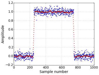
It is this sinc frequency response that makes the moving average a poor performer in the frequency domain. However, it performs very well in the time domain. Therefore, it is perfect to smooth data to remove noise while at the same time still keeping a fast step response (Figure 1).
 Figure 1. Smoothing with a moving average filter.
For the typical Additive White Gaussian Noise (AWGN) that is often assumed, averaging \(N\) samples has the effect of increasing the SNR by a factor of \(\sqrt N\). Since the noise for the individual samples is uncorrelated, there is no reason to treat each sample differently. Hence, the moving average, which gives each sample the same weight, will get rid of the maximum amount of noise for a given step response sharpness.
Implementation
Because it is a FIR filter, the moving average can be implemented through convolution. It will then have the same efficiency (or lack of it) as any other FIR filter. However, it can also be implemented recursively, in a very efficient way. It follows directly from the definition that
\[y[n+1]=y[n]+(x[n+1]-x[n-N+1])/N.\]
This formula is the result of the expressions for \(y[n]\) and \(y[n+1]\), i.e.,
\[y[n]=x[n-N+1]/N+\ldots+x[n]/N\]
and
\[y[n+1]=x[n-N+2]/N+\ldots+x[n+1]/N,\]
where we notice that the difference between \(y[n+1]\) and \(y[n]\) is that an extra term \(x[n+1]/N\) appears at the end, while the term \(x[n-N+1]/N\) is removed from the beginning. In practical applications, it is often possible to leave out the division by \(N\) for each term by compensating for the resulting gain of \(N\) in another place. This recursive implementation will be much faster than convolution. Each new value of \(y\) can be computed with only two additions, instead of the \(N\) additions that would be necessary for a straightforward implementation of the definition. One thing to look out for with a recursive implementation is that rounding errors will accumulate. This may or may not be a problem for your application, but it also implies that this recursive implementation will actually work better with an integer implementation than with floating-point numbers. This is quite unusual, since a floating point implementation is usually simpler.
The conclusion of all this must be that you should never underestimate the usefulness of the simple moving average filter in signal processing applications.
Filter Design Tool
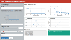
This article is complemented with a Filter Design tool. Experiment with different values for \(N\) and visualize the resulting filters. Try it now!

Hi Tom
I guess this is why Hogenauer Filter are called Cascaded Integrator Comb
Thank You Tom - you do a wonderful job
Benedito
Add new comment