Reconstruction of a Real Dataset, Part 2: Flat Field Correction

This is part two of a tutorial that describes how to create a reconstruction of a cone-beam computed tomography (CT) dataset (also read part one, part three, and part four). In this part, I’ll show how to preprocess the images to correct them for variations of the X-ray source intensity and of the detector sensitivity, the so-called flat-field correction.

The Problem

It would be easy if, for each pixel of the imaging system, the mathematical relation between the actual intensity of the X-rays and the output of the sensor would be

\[y=x,\]

for \(x\) the input and \(y\) the output. It would be equivalent to have a fixed gain \(g\) and a relation \(y=gx\), but we can just as well set \(g=1\).

However, there are two main effects to take into account to get the best possible results from the raw X-ray images. Using a linear model, which often seems sufficient, the relation between input and output can be written as

\[y=gx+b.\]

Dark Frames

The first effect that needs to be compensated for is the so-called dark current of the detector. The dark current is an electronic phenomenon that causes the detector pixels to report values different from zero, even when no X-ray photons are hitting it.

To measure the dark current, images are taken with the X-ray source turned off. These are called dark frames. Turning off the X-ray source implies that \(x=0\). Writing the equation of the imaging system while the dark frames are taken as \(d=gx+b\), setting \(x=0\) results in

\[d=b.\]

In other words, the dark frame immediately provides the contribution of the dark current of the detector.

For the whole detector, this results in a matrix \({\bf D}\). For the apple dataset, five dark-frame images were taken before the start of the scan. I have averaged those to create the final dark-frame image.

Flat Fields

The second effect is that the response to intensity variations is not the same for each detector pixel. In a normal digital camera this would be due to the optics and the detector. In the case of X-ray imaging there are typically no optics, but in addition to imperfections in the detector, there are effects such as the X-ray source being inhomogeneous.

To determine the response of the imaging system, a flat-field image is taken. The X-ray source is turned on, and an image is taken without an object present. Ideally, this would produce a perfectly homogeneous image. In practice it doesn’t, but the resulting image tells you exactly how “unflat” your X-ray imaging system is.

For the flat-field image, we set the input to a constant value, say, \(x=1\). While the flat fields are taken, the equation of the imaging system is \(f=gx+b\). Because we know that \(x=1\), we have that

\[f=g+b.\]

This results in \(g=f-b\). If we substitute that in \(y=gx+b\) and use that \(d=b\), we get

\[y=(f-d)x+d,\]

as the new equation of the imaging system, now written in function of the known values \(f\) and \(d\). The original input intensity \(x\) can then be computed from the measured pixel value \(y\) through

\[x=\frac{y-d}{f-d}.\]

For the whole detector, this again results in a matrix \({\bf F}\) for the flat-field image. For the apple dataset, 20 flat-field images were taken before the scan, and 20 after it. I have averaged those to get one “pre” and one “post” flat-field image.

Corrected X-Ray Image

For the whole detector, using \({\bf F}\) and \({\bf D}\), and using \({\bf X}\) for the actual intensities and \({\bf Y}\) for the output of the detector, the correction is

\[{\bf X}=\frac{{\bf Y}-{\bf D}}{{\bf F}-{\bf D}},\]

where all matrix operations are pixel wise.

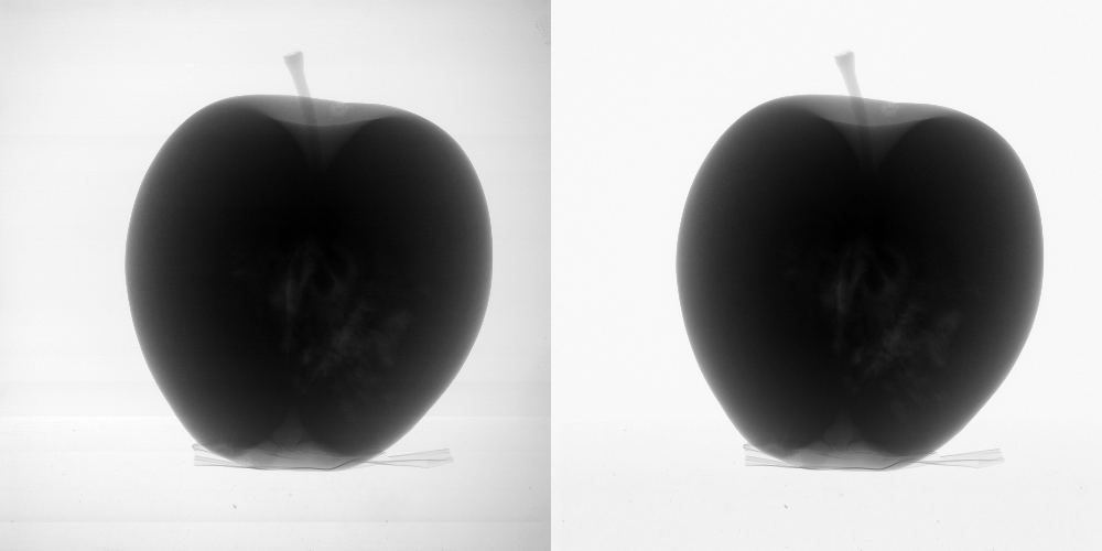
Figure 1 shows both a normalized version of the raw X-ray image from part one and a version corrected using the above formula, switching between the two every second. The correction clearly removes the vignetting (the reduction of the brighness in the corners) and the horizontal bands from the image.

Figure 1. Raw and corrected X-ray image.

The following is a technical detail, but I’ll share it anyway. With normalized raw X-ray image, I mean that the image is scaled to the same range of gray levels as the corrected image. This needs to be done to make the comparison useful. The difference is more spectacular without the normalization, but then it doesn’t clearly show the differences that actually matter anymore.

Part three of this tutorial shows how to turn these corrected X-ray images into projections, in the mathematical sense, so that they can be used for tomography. Part three also includes the Python code for these preprocessing steps.