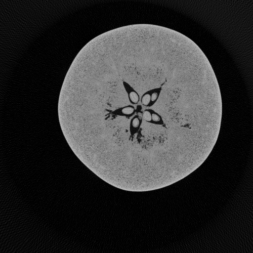
This is part four of a tutorial that describes how to create a reconstruction of a cone-beam computed tomography (CT) dataset (also read part one, part two, and part three). In this part, I’ll show how to create the actual reconstruction from the projections that were created in part three. To keep you in suspense no longer, Figure 1 shows the central slice of the reconstruction.
 Figure 1. Central slice of the reconstruction.
Python Code
The actual reconstruction code is very close to the code from ASTRA Toolbox Tutorial: Reconstruction from Projection Images, Part 2, so I won’t go into a lot of detail here, and go straight to the actual script! A few remarks follow.
- This script imports the file
config.pyfrom part one. - As for the code in ASTRA Toolbox Tutorial: Reconstruction from Projection Images, Part 2, you need an NVIDIA GPU to run this code, since the 3D algorithms of the ASTRA Toolbox are implemented as CUDA GPU code (for the previous parts of the current tutorial, a GPU or the ASTRA Toolbox were not required yet).
- As is often done, I have put the detector virtually in the origin of the coordinate system, so that it is in the center of the object. This means that the size of the detector pixels has to be adjusted, which is done in the computation of
detector_pixel_size_in_origin. - A funny statement is
im = np.roll(im, cfg.horizontal_shift, axis=1). This shifts each projection image two pixels to the left (the value ofcfg.horizontal_shiftis −2), to compensate for the axis of rotation not being entirely in the middle of the detector. This implementation is not entirely kosher, because therolloperation adds the two leftmost columns of the image to the right of the output image. This doesn’t make sense, but I can get away with it because there is only background in those columns. The ASTRA Toolbox allows you to do a direct adjustment of the geometry, which then also supports shifting by a fraction of a pixel, but I’ll keep that for a later post. - There is some postprocessing after the reconstruction. First I zero negative pixels. Then I compute the maximum using the central 200 slices. As for the code in part part three, the maximum is needed to create nicely scaled TIFF files. I use only the central 200 slices to avoid some bright spots in slices further away from the middle.
#filename: reconstruct.py
from __future__ import print_function
from __future__ import division

from os import makedirs
from os.path import join, exists
import numpy as np
from imageio import imread, get_writer

import astra
import config as cfg

def save_tiff(name, im_in):
    # Expects image as floating point in range [0, 1].
    im = im_in.copy()
    im = np.round(im * 65535).astype(np.uint16)
    with get_writer(name) as writer:
        writer.append_data(im, {'compress': 0})

if not exists(cfg.reco_dir):
    makedirs(cfg.reco_dir)

detector_pixel_size_in_origin = \
  cfg.detector_pixel_size * cfg.distance_source_origin / \
  (cfg.distance_source_origin + cfg.distance_origin_detector)

# Determine dimensions of projection images.
im = imread(join(cfg.proj_dir, 'proj0000.tif'))
dims = im.shape
# dims[0]: Number of rows in the projection image, i.e., the height of the
#          detector. This is Y in the Cartesian coordinate system.
# dims[1]: Number of columns in the projection image, i.e., the width of the
#          detector. This is X in the Cartesian coordinate system.
detector_rows = dims[0]
detector_columns = dims[1]

# Load projection images.
projections = np.zeros((detector_rows, cfg.num_projections, detector_columns))
for proj in range(cfg.num_projections):
    im = imread(join(cfg.proj_dir, 'proj{:04d}.tif'.format(proj))).astype(float)
    im /= 65535
    im = np.roll(im, cfg.horizontal_shift, axis=1)
    projections[:, proj, :] = im

# Copy projection images into ASTRA Toolbox.
proj_geom = astra.create_proj_geom('cone', 1, 1, detector_rows,
                                   detector_columns, cfg.angles,
                                   cfg.distance_source_origin /
                                   detector_pixel_size_in_origin, 0)
projections_id = astra.data3d.create('-sino', proj_geom, projections)

# Create reconstruction.
vol_geom = astra.creators.create_vol_geom(detector_columns, detector_columns,
                                          detector_rows)
reconstruction_id = astra.data3d.create('-vol', vol_geom, data=0)
alg_cfg = astra.astra_dict('FDK_CUDA')
alg_cfg['ProjectionDataId'] = projections_id
alg_cfg['ReconstructionDataId'] = reconstruction_id
algorithm_id = astra.algorithm.create(alg_cfg)
print('Reconstructing... ', end='')
astra.algorithm.run(algorithm_id)
print('done')
reconstruction = astra.data3d.get(reconstruction_id)

# Limit and scale reconstruction.
reconstruction[reconstruction < 0] = 0
middle = detector_rows // 2
M = np.max(reconstruction[middle - 100 : middle + 100, :, :])
reconstruction /= M
reconstruction[reconstruction > 1] = 1

# Save reconstruction.
for proj in range(detector_rows):
    print('Saving slice %d' % proj)
    slice = reconstruction[proj, :, :]
    save_tiff(join(cfg.reco_dir, 'reco%04d.tif' % proj), slice)

# Cleanup.
astra.algorithm.delete(algorithm_id)
astra.data3d.delete(reconstruction_id)
astra.data3d.delete(projections_id)
Download the Apple Dataset
If you think it would help you in understanding the code and applying it to your own datasets, I can actually provide you with the dataset that I’ve used in this series of articles! The nice people at UGCT, who created this dataset, have given me permission to make it available for download.
Simply shoot me a message and I’ll provide you with a download link (I don’t dare to put an actual download link here, since that might use a lot of bandwidth if it is linked from somewhere popular).
Hi Tom,
I´m working with 3d reconstruction and I´m searching some toolboxes for testing when I found this link.
Congrats for all your kindness explanations.
Best wishes...
Gustavo
Hi! Thanks for the nice tutorial. There is something I am curious about. How would I get the reconstructions in terms of Hounsfield units?
Hi! I am a new with 3D reconstruction. Your tutorial is very helpful to me.
Sincerely thanks for your tutorial.
Best wishes...
Chuck
Very nice tutorial
Add new comment