How to Create a Fractional-Delay Filter

With fractional delay, I mean a delay of a fraction of a sampling period. Introducing a delay of an integer number of samples is easy, since you can do that by simply skipping a number of samples, or buffering them if you don’t want to throw away a part of the signal.

As a practical example, take a digital signal that was sampled at a sampling rate of \(f_S=1000\,\mathrm{Hz}\). This means that a sample was taken every millisecond (the sampling period \(T=1/f_S=0.001\,\mathrm{s}\)). Delaying this signal by 3 ms is easy: skip 3 samples or insert a buffer that holds 3 samples in the processing chain. However, what to do if the signal must be delayed by 0.3 ms? That is the question that this article answers.

The Idea

The following technique for adding a fractional delay is based on the principle that a bandlimited signal that was correctly sampled can be reconstructed exactly. A signal is bandlimited if does not contain frequencies that are higher than a certain given frequency \(f\). If such a signal is sampled with a sampling rate \(f_S>2f\), then it can be reconstructed exactly. As I’ve already mentioned in Finite-Bandwidth Square Wave in Samples, this reconstruction can be done with the Whittaker–Shannon interpolation formula,

\[x(t)=\sum_{m=-\infty}^{\infty}x[m]\,{\rm sinc}\!\left(\frac{t-mT}{T}\right),\]

where the (normalized) sinc function is defined as

\[{\rm sinc}(t)=\frac{\sin \pi t}{\pi t}.\]

The output of the Whittaker–Shannon interpolation formula is the unique analog signal that corresponds to the given digital signal.

The idea behind introducing a fractional delay is now to first compute this analog signal, and then sample that again at the points in time that correspond with the required delay. It turns out that this can be done in a single step.

In Practice

First of all, since we are going to delay a digital signal, the actual value of \(T\) (or \(f_S\)) doesn’t matter, so we can set \(T=1\) for simplicity. This leads to

\[x(t)=\sum_{m=-\infty}^{\infty}x[m]\,{\rm sinc}(t-m).\]

Let’s use \(\tau\) for the fraction of a sample with which we want to delay the signal. To compute the delayed signal \(y[n]\), we compute \(x(t)\) for each point \(t=n-\tau\), as

\[y[n]=x(n-\tau)=\sum_{m=-\infty}^{\infty}x[m]\,{\rm sinc}(n-\tau-m).\]

Now compare this to the definition of (discrete) convolution,

\[(x*h)[n]=\sum_{m=-\infty}^\infty\!x[m]\,h[n-m].\]

It is clear that defining

\[h[n]={\rm sinc}(n-\tau)\]

and subsituting it into the definition of convolution leads to the expression for \(y[n]\) given above. This means that the delay operation can be implemented as a filter with coefficients \(h[n]\). We filter \(x[n]\) with \(h[n]\) to get the delayed signal \(y[n]\).

As for other sinc-based filters such as low-pass windowed-sinc filters, a remaining problem is that the sinc function has infinite support, which means that it cannot be used as-is, because that would result in an infinite delay. The solution for this is to window the coefficients. In the Python code that follows, I’ve used the well-known Blackman window to do that.

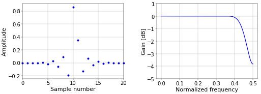
Figure 1 illustrates the impulse response and frequency response of a 0.3 samples delay filter with 21 coefficients that uses the above definition for \(h[n]\) (shifted to the range \([0,20]\) to make it causal), multiplied by a Blackman window.

Figure 1. Impulse response (left) and frequency response (right) of a 0.3 samples fractional delay filter with 21 coefficients.

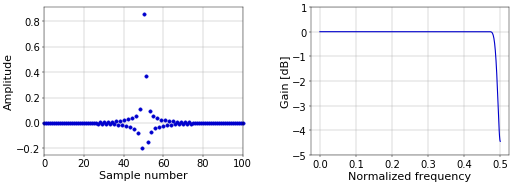
Changing the length of the filter has the effect of moving the point at which the frequency response starts to deteriorate. Figure 2 illustrates this with a filter with 101 coefficients.

Figure 1. Impulse response (left) and frequency response (right) of a 0.3 samples fractional delay filter with 101 coefficients.

Of course, these filters still have their standard delay of \((N-1)/2\) samples with \(N\) the length of the filter, in addition to the \(\tau\) samples delay (i.e., for \(N=21\) and \(\tau=0.3\), the total delay is \(10.3\) samples). Also note that you should keep \(\tau\) between \(-0.5\) and \(0.5\), to avoid making the filter more asymmetrical than it needs to be.

Python Code

The following Python program implements the filter of Figure 1.

from __future__ import division
 
import numpy as np
 
tau = 0.3  # Fractional delay [samples].
N = 21     # Filter length.
n = np.arange(N)
 
# Compute sinc filter.
h = np.sinc(n - (N - 1) / 2 - tau)
 
# Multiply sinc filter by window
h *= np.blackman(N)
 
# Normalize to get unity gain.
h /= np.sum(h)