Normalized Frequency For The Win

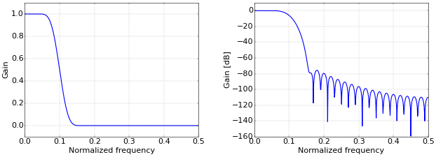
Frequency response plots are often shown with normalized frequency on the X-axis. This sometimes confuses people. Figure 1 shows the frequency response of a typical low-pass filter, taken from the article How to Create a Simple Low-Pass Filter.

Figure 1. Low-pass filter response with normalized frequency.

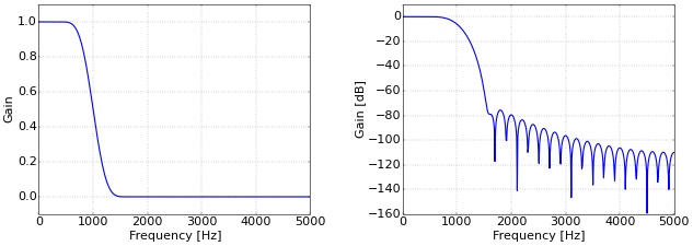
In this illustration, the range of the normalized frequency is [0, 0.5]. The normalized frequency is computed by dividing the true frequency by the sampling rate. Hence, the sampling rate itself has a normalized frequency of one. However, a digital signal can only uniquely represent frequencies up to half the sampling rate (the Nyquist frequency), which makes the practical limit 0.5. Many people might argue that the plots in Figure 2 are easier to interpret (the difference is in the scale of the X-axis).

Figure 2. Low-pass filter response with true frequency.

And many people might be right. The second pair of plots shows the frequency response of the filter for a sampling rate of 10 kHz. This makes the cutoff frequency of the filter, which is 1 kHz, immediately clear. However, the danger is that a graph like this could be interpreted as “this filter removes frequencies above 1 kHz”, while the correct interpretation is “at a sampling rate of 10 kHz, this filter removes frequencies above 1 kHz”. In practice, a digital filter is applied to a series of numbers, and the sampling rate at which these numbers were acquired is nowhere in sight. If, for example, the filter from Figure 2 would be applied to a signal that was sampled at 20 kHz, the cutoff point of the filter would quietly change to 2 kHz.

Hence, it is more logical and less confusing to use the first pair of graphs instead, where only the normalized frequency is shown. So, if you read articles such as How to Create Simple Band-Pass and Band-Reject Filters, apply them to the problem at hand by multiplying the normalized frequency with the sampling rate to get the practical effect of the filter.