In earlier posts, I’ve introduced both windowed-sinc filters (low pass, high pass, and band pass and band reject) and the moving average as a filter. Windowed-sinc filters are very good in the frequency domain, i.e., they are very good at “doing different things with different frequencies”. Typical examples are removing certain frequencies, as a low-pass filter does, or equalization in audio applications. The moving average, on the other hand, is very good in the time domain. Its main application is reducing random noise.
In the mentioned articles, I’ve mainly stressed the properties of these filters in the domain in which they perform strongly. In this article, I’ll also show their performance in the other domain.
Windowed-Sinc Filters
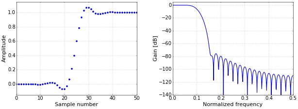
Figure 1 shows the step response of the low-pass windowed-sinc filter of How to Create a Simple Low-Pass Filter, next to its frequency response.
 Figure 1. Windowed-sinc step (left) and frequency (right) responses.
It is clear that this filter is very good in separating different frequencies. The roll-off is sharp, and can be made almost arbitrarily sharper by increasing the length of the filter. Equally important, the suppression of the unwanted frequencies is very good, and can be increased further by applying the filter several times, or, equivalently, by convolving the filter kernel with itself to create a new filter.
However, the performance of the windowed-sinc filter in the time domain is not so good. At sudden changes in the signal level, windowed-sinc filters produce unwanted oscillations known as ringing, and overshoot. Hence, if the information in your signal is in the time domain, you need a different type of filter. Note that the step response that is shown in Figure 1 is completely equivalent to the impulse response, since it is simply the cumulative sum of the impulse response. However, the step response is better suited to illustrate the time domain performance of the filter, since it shows how the filter interacts with an “edge” in the signal.
Moving-Average Filters
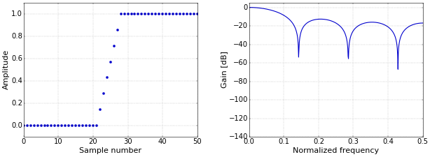
The basic filter to use if the information in your signal is in the time domain, is the moving-average filter. Figure 2 shows the step and frequency response of a moving average filter of length 7. Note that the horizontal segments in the step response plot are not really part of the step response, but only included for clarity. I’ve picked a length of 7 so that the rise time is comparable with that of the windowed-sinc filter of Figure 1.
 Figure 2. Moving-average step (left) and frequency (right) responses.
The moving-average filter is clearly very bad at separating frequencies. Additionally, we can pick a cutoff frequency for a windowed-sinc filter (set to 0.1 for the filter of Figure 1), which we can’t do for the moving average.
However, the time domain performance of the moving average, for suppressing as much noise as possible, is perfect. To reiterate what I’ve already mentioned in the article on the moving-average filter, for Additive White Gaussian Noise (AWGN), averaging \(N\) samples has the effect of increasing the SNR by a factor of \(\sqrt N\). And, since the noise for the individual samples is uncorrelated, there is no reason to treat each sample differently. Hence, the moving average, which gives each sample the same weight, will get rid of the maximum amount of noise for a given step response sharpness.
In conclusion, when picking a filter, it is important to clearly decide where the useful information in your signal is. If the information is in the frequency domain, it might be best to start with a windowed-sinc filter. If the information is in the time domain, the simple moving average might be perfect. In a future article, I’ll describe a few variations of the moving average that might be useful if you are working with a mixed-domain signal.
Filter Design Tool
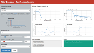
This article is complemented with a Filter Design tool. Experiment with different settings, visualize the resulting filters, and download the filter coefficients. Try it now!

Add new comment