This article shows how “old style” linear regression looks when implemented with TensorFlow. When you start diving into TensorFlow, an example like this is typically missing from the tutorials. Linear regression is often the first example, but the tutorials immediately start from datasets with the normal machine learning terminology such as feature and label. If you’ve used linear regression before, this can make it a bit difficult to see the basic operation of the algorithm, not because it is different from linear regression, but because of the new terminology and typical machine learning approach. Hence, this little article tries to “map” classical linear regression to the same thing in TensorFlow. If you are a machine learning expert, for heaven’s sake stop reading now, before your mind becomes irrevocably corrupted by this old style stuff!
The script below starts from two NumPy arrays x and y representing \(n\) data pairs \((x_i, y_i\)). Using the equation of a line, \(y=wx+b\), linear regression starts from the relation \(y_i=wx_i+b+e_i\), where each pair \((x_i, y_i)\) results in a specific error \(e_i\). It then solves for the parameters \(w\) and \(b\) that minimize the error terms \(e_i\), typically by determining those values for \(w\) and \(b\) so that the sum of squares of \(e_i\), \(\sum_{i=1}^{n}e_i^2\), is minimized. Using SciPy and classical linear regression, you could write something like from scipy.stats import linregress; w, b = linregress(x, y)[0 : 2].
To map this to TensorFlow, you make x the features and y the labels. I’ve used the high-level Estimator TensorFlow API for this example. Because the estimator assumes that its data is produced by an input function, you have to define a function such as input_fn() in the code below. This particular implementation simply returns the full arrays x and y. This means that the script will do batch gradient descent, i.e., that the complete input dataset is used in each step of the optimization.
import numpy as np
import tensorflow as tf

n = 150
x = np.random.rand(n) * 4 - 2
y = x + np.random.randn(n) * 0.2 + 0.1

def input_fn():
    features = {'x': x}
    labels = y
    return features, labels

xfc = tf.feature_column.numeric_column('x')
estimator = tf.estimator.LinearRegressor(feature_columns=[xfc])
estimator.train(input_fn=input_fn, steps=100)

w = estimator.get_variable_value('linear/linear_model/x/weights')[0][0]
b = estimator.get_variable_value('linear/linear_model/bias_weights')[0]
If you call the estimator.train() function with steps=100, then the complete dataset of 150 points is used 100 times. When the function returns, the values for \(w\) and \(b\) can be retrieved through calls to the function estimator.get_variable_value(), as shown in the code. For a new value of \(x\) that was not in the original data, you can then compute \(y\) by using the equation \(y=wx+b\). And, in this way, you have done classical linear regression with TensorFlow!
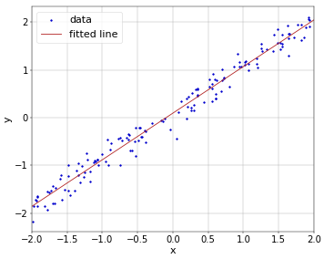
As an illustration, the data points and fitted line for an example run of the above Python script are shown in Figure 1.
 Figure 1. Line fitted through linear regression.
I am new to tensor flow. is it correct to assume that the 'training' in yr example is done iteratively via eg gradient descent, rather than the deterministic normal equation approach ?
Indeed, it uses one of several supported variants of gradient descent. It uses all data points in each iteration, so this would be batch gradient descent. More typical for machine learning is stochastic (one data point per iteration) or mini-batch gradient descent (in-between both).
Thank you very much, I was looking for exactly this kind of solution, The most common solution out there is using TensorFlow low-level API by defining Tensors, but it's taking so long to converge.
Add new comment