Summary: This article shows how to implement a low-pass single-pole IIR filter. The article is complemented by a Filter Design tool that allows you to create your own custom versions of the example filter that is shown below.
The low-pass single-pole IIR filter is a very useful tool to have in your DSP toolbox. Its performance in the frequency domain may not be stellar, but it is very computationally efficient.
Definition
A low-pass single-pole IIR filter has a single design parameter, which is the decay value \(d\). It is customary to define parameters \(a=d\) and \(b=1-d\) (the logic behind this follows from the general case below). For a typical value of \(d=0.99\), we have that \(a=0.99\) and \(b=0.01\). The recurrence relation is then given by
\[y[n]=bx[n]+ay[n-1],\]
where the sequence \(x[n]\) is the input and \(y[n]\) is the output of the filter.
The recurrence relation directly shows the effect of the filter. The previous output value of the the filter, \(y[n-1]\), is decreased with the decay factor \(a=d\). The current input value, \(x[n]\), is taken into account by adding a small fraction \(b=1-d\) of it to the output value.
Substituting \(b=1-a\) in the given recurrence relation and rewriting leads to the expression
\[y[n]=y[n-1]+b(x[n]-y[n-1]).\]
This then leads to compact update expressions such as y += b * (x - y), in programming languages that support the +=-operator (see the Python code below for an example).
Impulse Response
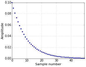
For windowed-sinc filters (see, e.g., How to Create a Simple Low-Pass Filter), the impulse response is the filter. To apply the filter, you convolve the impulse response of the filter with the data. This is different for the single-pole IIR filter. Its action is essentially defined on a sample-by-sample basis, as described by the recurrence relation given above. The impulse response of a filter with \(d=0.9\) (\(b=0.1\)) is shown in Figure 1.
 Figure 1. Impulse response of a low-pass single-pole filter.
Of course, this impulse response is actually infinite. I’ve plotted the first 50 samples here, and at that point it is quite close to zero, but it never actually reaches zero.
Properties
The response of this filter is completely analogous to the response of an electronic low-pass filter consisting of a single resistor and a single capacitor.
The decay value \(d\) is related to the time constant \(\tau\) of the filter with the relation
\[d=e^{-1/\tau}.\]
Hence, if \(d\) is given, the value of \(\tau\) can be computed as \(\tau=-1/\ln(d)\). As for an electronic RC-filter, the time constant \(\tau\) gives the time (in samples for the discrete case) for the output to decrease to 36.8% (\(1/e\)) of the original value.
Another useful relation is that between \(d\) and the (-3 dB) cutoff frequency \(f_c\), which is
\[d=e^{-2\pi f_c}.\]
Hence, if \(d\) is given, the value of \(f_c\) can be computed as \(f_c=-\ln(d)/2\pi\).
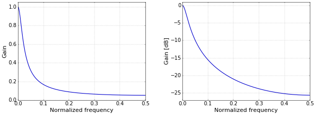
The frequency response of the filter with the impulse response of Figure 1 is given in Figure 2.
 Figure 2.Frequency response on a linear (left) and logarithmic (right) scale.
Python code
In Python and in most other programming languages, the recurrence relation can be implemented through the already mentioned expression y += b * (x - y). Below is a small Python class that implements this expression in its filter() member.
decay = 0.9  # Decay between samples (in (0, 1)).

class LowPassSinglePole:
    def __init__(self, decay):
        self.b = 1 - decay
        self.reset()
    def reset(self):
        self.y = 0
    def filter(self, x):
        self.y += self.b * (x - self.y)
        return self.y

low_pass_single_pole = LowPassSinglePole(decay)
This filter can then be applied by calling the filter() member for each new input sample x, resulting in a new output sample y:
y = low_pass_single_pole.filter(x)
Filter Design Tool
This article is complemented with a Filter Design tool. Experiment with different values for \(d\), visualize the resulting filters, and download the filter code. Try it now!
General Case
This last section is mainly here to have everything in one place for now. I plan to add a separate article on the Z-transform later.
A single-pole low-pass infinite impulse response (IIR) filter is given by the Z-transform
\[H[z]=\frac{bz}{z-a}=\frac{b}{1-az^{-1}},\]
where \(a+b=1\) results in a filter with unity gain at DC.
The general form of this equation is
\[H[z]=\frac{b_0+b_1z^{-1}+b_2z^{-2}+\ldots}{1-a_1z^{-1}-a_2z^{-2}+\ldots}=\frac{\sum\limits_{n=0}^{\infty}b_nz^{-n}}{1-\sum\limits_{n=1}^{\infty}a_nz^{-n}}.\]

"where a+b=1 results in a filter with unity gain." Should be "... unity gain at DC."
Yes, at DC. I’ve added it in the article for completeness.
Hi!
I've encountered two conflicting formulas for the decay coefficient and decided to ask about that on Stack Exchange.
The formula you provide is an approximation, see https://dsp.stackexchange.com/questions/54086/single-pole-iir-low-pass-….
It seems to work fine with lower frequencies, but its value differs significantly when the center frequency is too high.
Thanks for your attention! :)
Indeed, it's an approximation. Maybe I should have mentioned that. In practice, however, I think that this filter is often used with relatively small cutoff frequencies. For example, for d=0.99, the (estimated) cutoff frequency is about 0.0016 (relative to 0.5; the plot in the StackExchange answer that you refer to is relative to 1), which is clearly in the usable range of the approximation.
Thank you for this article. As an absolute amateur in DSP I found it very helpful.
Can you comment on the group delay of the one pole filters?
I'll consider adding an article on group delay, because that is indeed missing for now...
Thank you. I was using a sensor change detection routine in Arduino for my music keyboard that uses analog sensors in every key, instead of double or triple switches per key, but the filter is much more better and accurate since it doesn't skip any values.
If you want to compare between the two, see the code below..
Add new comment