Summary: This article shows how to create a simple low-pass filter, starting from a cutoff frequency \(f_c\) and a transition bandwidth \(b\). This article is complemented by a Filter Design tool that allows you to create your own custom versions of the example filter that is shown below, and download the resulting filter coefficients.
How to create a simple low-pass filter? A low-pass filter is meant to allow low frequencies to pass, but to stop high frequencies. Theoretically, the ideal (i.e., perfect) low-pass filter is the sinc filter. The sinc function (normalized, hence the \(\pi\)’s, as is customary in signal processing), is defined as
\[\mathrm{sinc}(x)=\frac{\sin(\pi x)}{\pi x}.\]
The sinc filter is a scaled version of this that I’ll define below. When convolved with an input signal, the sinc filter results in an output signal in which the frequencies up to the cutoff frequency are all included, and the higher frequencies are all blocked. This is because the sinc function is the inverse Fourier transform of the rectangular function. Multiplying the frequency representation of a signal by a rectangular function can be used to generate the ideal frequency response, since it completely removes the frequencies above the cutoff point. And, since multiplication in the frequency domain is equivalent with convolution in the time domain, the sinc filter has exactly the same effect.
The windowed-sinc filter that is described in this article is an example of a Finite Impulse Response (FIR) filter.
Sinc Filter
The sinc function must be scaled and sampled to create a sequence and turn it into a (digital) filter. The impulse response of the sinc filter is defined as
\[h[n]=2f_c\mathrm{sinc}(2f_cn),\]
where \(f_c\) is the cutoff frequency. The cutoff frequency should be specified as a fraction of the sampling rate. For example, if the sampling rate is 10 kHz, then \(f_c=0.1\) will result in the frequencies above 1 kHz being removed. The central part of a sinc filter with \(f_c=0.1\) is illustrated in Figure 1.
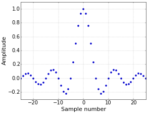 Figure 1. Sinc filter.
The problem with the sinc filter is that it has an infinite length, in the sense that its values do not drop to zero. This means that the delay of the filter will also be infinite, making this filter unrealizable. The straightforward solution is to simply stop computing at a certain point (effectively truncating the filter), but that produces excessive ripple. A better solution is to window the sinc filter, which results in, you guessed it, a windowed-sinc filter.
Window
A window function is a function that is zero outside of some interval. There exist a great variety of these functions, tuned for different properties, but I’ll simply use the well-known Blackman window here, which is a good choice for general usage. It is defined as (for \(N\) points)
\[w[n]=0.42-0.5\cos\left({\frac{2\pi n}{N-1}}\right)+0.08\cos\left({\frac{4\pi n}{N-1}}\right),\]
with \(n\in[0,\,N-1]\). It is shown in Figure 2, for \(N=51\).
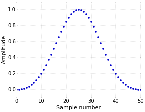 Figure 2. Blackman window.
Windowed-Sinc Filter
The final windowed-sinc filter is then simply the product of the two preceding expressions, as follows (with the sinc filter shifted to the range \([0,\,N-1]\)).
\[h[n]=\mathrm{sinc}\left(2f_c\left(n-\frac{N-1}{2}\right)\right)\left(0.42-0.5\cos\left({\frac{2\pi n}{N-1}}\right)+0.08\cos\left({\frac{4\pi n}{N-1}}\right)\right),\]
with \(h[n]=0\) for \(n\notin[0,\,N-1]\). I have dropped the factor \(2f_c\) from the sinc filter, since it is much easier to ignore constants at first and normalize the complete filter at the very end, by simply making sure that the sum of all coefficients is one, giving the filter unity gain, with
\[h_\mathrm{normalized}[n]=h[n]/\sum_{i=0}^{N-1}h[i].\]
This results in the normalized windowed-sinc filter of Figure 3.
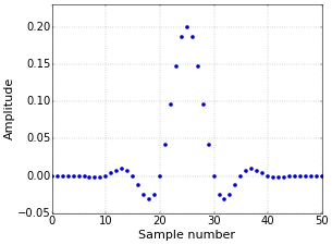 Figure 3. Normalized windowed-sinc filter.
Transition Bandwidth
The final task is to incorporate the desired transition bandwidth (or roll-off) of the filter. To keep things simple, you can use the following approximation of the relation between the transition bandwidth \(b\) and the filter length \(N\),
\[b\approx\frac{4}{N},\]
with the additional condition that it is best to make \(N\) odd. This is not really required, but an odd-length symmetrical FIR filter has a delay that is an integer number of samples, which makes it easy to compare the filtered signal with the original one. Setting \(N=51\) above was reached by setting \(b=0.08\). As for \(f_c\), the parameter \(b\) should be specified as a fraction of the sampling rate. Hence, for a sampling rate of 10 kHz, setting \(b=0.08\) results in a transition bandwidth of about 800 Hz, which means that the filter transitions from letting through frequencies to blocking them over a range of about 800 Hz. The values for \(f_c\) and \(b\) in this article were chosen to make the figures as clear as possible. The frequency response of the final filter (with \(f_c=0.1\) and \(b=0.08\)) is shown in Figure 4.
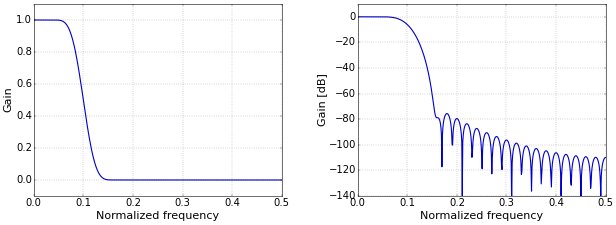 Figure 4. Frequency response on a linear (left) and logarithmic (right) scale.
Python Code
In Python, all these formulas can be implemented concisely.
from __future__ import division

import numpy as np

fc = 0.1  # Cutoff frequency as a fraction of the sampling rate (in (0, 0.5)).
b = 0.08  # Transition band, as a fraction of the sampling rate (in (0, 0.5)).
N = int(np.ceil((4 / b)))
if not N % 2: N += 1  # Make sure that N is odd.
n = np.arange(N)

# Compute sinc filter.
h = np.sinc(2 * fc * (n - (N - 1) / 2))

# Compute Blackman window.
w = 0.42 - 0.5 * np.cos(2 * np.pi * n / (N - 1)) + \
    0.08 * np.cos(4 * np.pi * n / (N - 1))

# Multiply sinc filter by window.
h = h * w

# Normalize to get unity gain.
h = h / np.sum(h)
Applying the filter \(h\) to a signal \(s\) by convolving both sequences can then be as simple as writing the single line:
s = np.convolve(s, h)
In the Python script above, I compute everything in full to show you exactly what happens, but, in practice, shortcuts are available. For example, the Blackman window can be computed with w = np.blackman(N).
In the follow-up article How to Create a Simple High-Pass Filter, I convert this low-pass filter into a high-pass one using spectral inversion. Both kinds of filters are then combined in How to Create Simple Band-Pass and Band-Reject Filters
Filter Design Tool
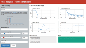
This article is complemented with a Filter Design tool. Experiment with different values for \(f_c\) and \(b\), visualize the resulting filters, and download the filter coefficients. Try it now!
Thanks! That's a very useful article.
Could you explain, what can I do with delay between source and filtered signals?
The nice thing about these kinds of filters is that it is easy to compensate for their delay. Symmetrical FIR filters, of which the presented windowed-sinc filter is an example, delay all frequency components in the same way. This means that the delay can be characterized by a single number. The delay of a filter of length M equals (M-1)/2. Hence, the shown filter with 51 coefficients has a delay of exactly 25 samples. So, if you want to overlay the original signal with the filtered one to compare them, you just need to shift one of them by 25 samples!
I don't understand how to compensate for the signal delay so that the signal matches the source signal.
If the delay is 25 samples, as in the example, then you can simply remove the first 25 samples of the filtered signal, or add 25 zeros at the beginning of the original signal. If you do that, and you plot the two signals on top of each other, then there will be no delay between them anymore.
Really appreciate how concise this article is. Thanks!
Thank you! It's a very nice article. Could you maybe explain why it is necessary to normalize each element in h by the sum(h)?
It’s not really necessary, but if you make sure that the sum of the coefficients is one, then the gain of the filter at DC is also one. Additionally, it allows you to make the gain of the filter whatever you want simply by multiplying the coefficients of the normalized filter by the required gain factor.
Thanks very much for your article... I had considered this topic whole week and now my mind is clear!
Thanks, this is really helpful !
Great article!
How do you make your plots?
Thanks
Thanks! The plots for most of the articles, including this one, were made with Python (using matplotlib).
Very interesting and clear article, thanks Tom! Question: You say that the number of coefficients is approx 4/b. If i use your fir designer tool and design a lowpass (windowed sinc) with Samplerate=44100, Cutoff=1000, Bandwidth=1000, i would expect approx 4/(1000/44100) = 176.4 thus 177 coefficients, but it gives 203 coefficients. I have been searching for the logic in that but i don't understand it. How do you define the specific number of coefficients? Thanks.
That’s a good observation. The reason for this is that the number of coefficients in the tool depends on the window function. This is because the window has a large influence on the transition bandwidth, so that, e.g., the rectangular window can get by with much less coefficients than the Blackman window. Maybe I'll write a separate article on this with more details, because it’s quite interesting stuff. In practice, the tool uses 4.6/b for Blackman, 3.1/b for Hamming, and 0.91/b for rectangular. From your example, I can tell that you’ve used a Blackman window, since 4.6/(1000/44100) = 202.86.
In the meantime, I’ve added the article The Transition Bandwidth of a Filter Depends on the Window Type with more details on this.
Thanks for your tutorial, well detailed!
Is the signal that you filter an array containing the amplitude of the signal?
Thanks! And yes, the variable
sin the example is an array of numbers. I would say that this is the signal, and not just its amplitude.Hi, Can you explain why its not just the amplitudes?
Great articles, thank you very much!
I was just being nitpicky a bit, I think... :-) The signal is indeed really just a series of numbers that represent an amplitude. It’s just that saying “the amplitude of the signal” could suggest that you’ve left something out or did some sort of preprocessing. That’s why I’d just write “the signal”…
Thanks for this great article. I have a question regarding Figure 4. How did you create the frequency response diagram?
This is another great idea for a follow-up article! I'll do one where I explain this in detail. In short, you first pad the filter with zeros to increase the resolution of the frequency plot, then take an fft, compute the power, and plot the result, either on a linear scale or in dB.
In the meantime, I've written an article that shows exactly how I typically plot the frequency response of a filter.
Thank you. Would you write something about IIR?
Currently, I indeed only have an article on the (important) low-pass single-pole IIR filter. Are there any specific things on IIR filters or filter types that you would find interesting?
Well-elaborated! Many thanks.
This was very useful, thanks!
Hello, i'm implementing a fir filter, band reject to be exact, could the signal s be the data of an fft from an audio.wav?
Your signal
sshould be the data of the audio.wav file, not the FFT of the data. Of course, if you are going to implement the convolution in the frequency domain, then you need to take the FFT of both the signal and the filter coefficients.Sorry Tom,
I was wrong in my earlier comment. fS/fL evaluates to zero in Python 3 as well, so the code gives the Blackman weights.
Your plots are, of course, correct but the display maybe doesn't come from the sample code shown below ?
I am a geophysicist, seismic sampling is often 500 -1000Hz The input box is labelled Hz.
Once again, thanks !
very impressive !
Jim
______________________________
import numpy as np
# Example code, computes the coefficients of a low-pass windowed-sinc filter.
# Configuration.
fS = 1000 # Sampling rate, ***** works fS = 1000.0 ? *****
fL = 20 # Cutoff frequency, *****works fL = 20.0 ? *****
N = 461 # Filter length, must be odd.
# Compute sinc filter.
h = np.sinc(2 * fL / fS * (np.arange(N) - (N - 1) / 2.))
# Apply window.
h *= np.blackman(N)
# Normalize to get unity gain.
h /= np.sum(h)
print(h)
# Applying the filter to a signal s can be as simple as writing
# s = np.convolve(s, h)
Hello Jim,
fL/fS (or fS/fL) does definitely not evaluate to zero in Python 3. Maybe two version of Python are installed on your computer, and you're still using Python 2? The plots on fiiir.com are indeed not generated in Python.
Tom
Tom,
Yes, indeed, I did have both versions active and must have used 2.7 again.
I just ran it in Python 3.4.5 and it works fine, a lesson learned.
I should have checked, was confused debugging in Idle
Jim
Awesome! you made windowed-sinc-filter design very easy!
Hi Tom,
I'm trying to apply this filter to my data which has sample rate of 250Hz and contains 1000 samples. After applying the filter my data has 1050 samples instead of 1000. Am I doing something wrong? Please help.
Thanks in advance.
This is normal. The length of the output signal is the length of the input signal plus the length of the filter minus one. This follows from the definition of convolution, but for a more intuitive understanding, have a look at the nice animations on https://en.wikipedia.org/wiki/Convolution#Visual_explanation. An effect of this is that you will see a so-called transient response of the filter in the beginning of your output signal, and that you have to wait a number of samples (the length of the filter, i.e., 51 samples in case of the example filter) before the filter is "filled up" and you get the actual response for which the filter was designed (the so-called steady state response).
Thanks Tom. I understand it better now.
I found it myself :). That was due to numpy.convolve. I used mode='same' and I got what I want.
Very good article.
Thanks for the articale and online filter-designer!
But it seems to me there must bу 2. * fL шт formula:
h = np.sinc(2 * fL / fS * (np.arange(N) - (N - 1) / 2.))
Ran it on Python 2.7 and found out with integer 2 the filter coefficients differ drastically (but with float 2, they correspond to the generated in pyhon list).
Thanks for pointing this out! (For other readers, the code snipped is from one of the generated Python programs from fiiir.com.) I've assumed Python 3 for a long time for all code on this site and on fiiir.com (you know, looking towards the future and all), but I think that I'll have to fold and make all my code compatible with both Python 2 and Python 3, because people keep reporting these kinds of problems… I'll look into it…
The code is now fully compatible with both Python 2 and Python 3. I've added
from __future__ import division(see One Code to Run Them All (Python 2 and Python 3) for details).Thanks for your article.
That's a very useful article.
Could you explain, could we define this(=low_pass_filter) as one of FFT filters?
I saw someone called it(=low_pass_filter) as one of FFT filters.
Sorry for my English.
Yes, you can use FFT convolution with these filters, with exactly the same result. Instead of applying the filter with
s = np.convolve(s, h)as described above, you could usefrom fft.signal import fftconvolves = fftconvolve(s, h)According to the documentation for SciPy fftconvolve(), the SciPy
convolve()even picks the best algorithm (direct or FFT) automatically. The NumPyconvolve()that I've used above doesn't do that.Hi Tom,
Thanks for the article. How would you determine the transition band width of Kaiser window function? Is it possible to provide the article where you found the transition band width for other window functions? And what is the criteria to determine the cutoff frequency? Thank you in advance!
I might misunderstand your question, but the cutoff frequency and rolloff normally follow from the problem that you are trying to solve by applying the filter that is being designed. For example, if the useful signal in the input has low frequencies and there is high frequency interference, then you could put the cutoff frequency "halfway" and make the rolloff as large as possible (to make the filter shorter) without removing part of the signal or letting through part of the noise.
I don't remember where I got the values for the other window functions… For (some) more details, see The Transition Bandwidth of a Filter Depends on the Window Type).
Thank you for the response, Tom. I am doing a lab experience, so I need to find a way to determine the cutoff frequency and rolloff parameters. I am new for signal processing, so I'm not quite sure the limitation to determine the parameters. When you say to make the rolloff as large as possible, is that mean to make the transition bandwith is smaller (the slope is steeper)?
As large as possible means to make the transition bandwitdh larger, so the that the slope is less steep. The effect of this is that the filter becomes shorter (has less coefficients). This can be important if you have large amounts of data or for real-time processing, because a short filter can be faster to compute (depending on its implementation). You can play with this on fiiir.com. To determine the cutoff frequency and rolloff, you have to look at your data: which frequencies do you want to let through, and which ones do you want to block? That's what will determine your choice of parameters.
I am a bit confused. I thought an ideal case for the filter is when it has a straight down transition bandwidth (zero width), which means we need the roll-off as narrow as possible, thus the slope is steeper. This can increase the signal-to-noise ratio. Am I misunderstanding the terminologies? Thanks!
It all depends on your input signal: the rolloff only needs to be steep enough to filter out the unwanted frequencies. It's fine if it's steeper, but then your filter will be longer…
thank you TomRoelandts. the article really help.
Hi. I want to convolve an image with sinc(t) function for t>0. Does anyone can help me how I should do that?
Thanks for this. I was looking for the relation between cutoff freq and the sinc function on FIR filters and it was not until I found this that doubts disappeared. cheers
Hi, Tom:) I just took a General Education course on sound and music and wanted to create a talk about subtractive synthesis and this lowpass filter in code will really help my presentation! Thanks a lot! but for some reason, i cant seem to apply the filter to any music clips or any soundwaves i generate. There are many errors that are being thrown up. is it possible for you to show a sample of how to apply it to a sound clip that you can easily find from anywhere ie Youtube?
Hello Sean, This is a completely different problem from the filtering operation itself, of course. The thought of adding a post on this more technical aspect of audio processing has crossed my mind, but I am currently very busy professionally and don't have a lot of spare time for things like that. My advise would be to start by writing a Python program that reads an audio file, converts it to floating point numbers, converts it to integers again, and then writes it to a different file. If that works without problems, then adding the filter will be easy...
Hello Tom ! I used your FIIIR tools in order to construct some anti-aliasing filter. But I have some problems when the cut-off frequency is small for example I have a nice 81 pts FIR sinc*blackman with parameters (sampling rate;cut-off_freq;transition) = (1;0.25;0.0575) :) But when I want upsampling for example with a factor 10 (in order to apply a lowpass filter and decimate with a filter (sampling rate;cut-off_freq;transition) = (1;0.025;0.0575) the filter seems to become smooth in frequency domain. Is it normal ? Can't we preserve the sharp-cut off ?
Hi, Tom
Thanks very much for this useful site to design a low pass filter.
I am using this online tool for an audio stream of which sampling rate is 384KHz.
I need to cut off the stream around 300Hz - 1KHz. However, your tool allows the lowest cutoff frequency as low as 10% of the sampling rate, that is 3840Hz.
I wonder why there is such limitation in your tool. Is it the limit of a low pass FIR filter? And it would be much appreciated if you suggest how to get the coefficients for the filter with lower cutoff frequency.
Thank you again for this useful site.
Best regards,
Jason.
It's 1%, of course. But you are right that the limit is arbitrary. However, there is a practical reason: The length of the filter is determined by the transition bandwidth, and I wanted to keep that length under 1000 (also for band-pass filters), so I set the limit of the transition bandwidth to 0.01. And then it doesn't make sense to allow a cutoff frequency that is much smaller…
As a practical solution, you could use the Python code from the this article directly. That has no such arbitrary limit.
Another option, to avoid that your filters become very long, is to filter in stages and subsample (i.e., throw away samples) in between stages.
Wow you explained very well. May I ask about window selection? How is it different if we only know the sampling rate? So what's the difference in deciding which window to choose?
The window selection depends on the application that the filter is designed for. For example, say that you need to suppress the high frequencies by a certain number of dB, but you want the filter to be as short as possible for performance reasons (in the sense of CPU usage). You could then use a Kaiser window and experiment with the least amout of suppression that you can get away with. There are many other window types that were designed so that the ouput has properties that are useful for specific applications.
Hi Tom!
First of all, thanks for these filters, they do work really well :)
I have a question for you,
Made a low-pass filter for 44100Hhz, cutoff at 11025Hz, transition at 441Hz, Blackman, i.e. the best possible to sound like as if at 22050Hz.
The CPU usage skyrocketed to 50%, I somehow managed to get that down to 35% by profiling and fixing everything I could on my side outside of the convolution process itself.
Was wondering if there would be some "silver bullet" in regard to further improve the convolution process itself.
I know I'm asking for the moon but who knows, maybe you have some trick up your sleeve to share with us!
Thanks :D
Never mind, I figured it out, rewrote the algorithm in native code and CPU usage is now ~4% 😍!
I was still going to answer, but I was too slow... :-)
Another suggestion might be to use FFT convolution (I already mention it in a comment above). Whether it's worth it depends on the length of the filter, and it takes extra work if you have a continuous stream of samples, but it can boost performance a lot in many cases. In Python it's easy, but in C/C++ you'll need something like FFTW (https://www.fftw.org/).
But with 4% of CPU usage, you probably don't care to much anymore... :-)
I didn't notice you replied, I checked my mailbox but I can't see any notification anywhere...
Now I am facing a dilemma with your answer, since last time I managed to further crank it up by 100%, it's about 0.2ms and 2% CPU now. I learned about half-band filters and realized that it actually is one; tried that among doubling delay line and processing whole chunks instead, speed doubled immediately.
I was all happy with green indicators all around then you dropped the FFT bomb... I "heard" about it but deemed it might be overkill since I'm processing lots of small buffers. But well, after looking closely, it appears that I'm wrong and that it is on an another level! I guess I'm going to give it a try...🤣
In that case, my main suggestion would be to try it in Python first and see whether it makes a big difference for the size of your filter. The NumPy functions such as convolve are actually implemented in C, so Python can be used to judge whether switching to fftconvolve is worth it...
I hate to admit defeat but in that case I'm going to have to! 🏳️😂
I looked at FFT convolution but couldn't find an example about an algorithm that handles chunks using overlapping. That threw me off because it's clear I'm not going to figure it out in a reasonable time.
Then I'd have to bring a good FFT library. For this, I'd have to auto-generate bindings so I can use them in Unity. Experience shown it's long to do and doing it by hand is a no-go since it's really error-prone.
Finally, rewrote my code to see that going all native code is useless as it didn't improve (only convolution does) and profiled again to see that it goes between 0.9% CPU and 2.8% CPU, i.e. external factors.
So I weighted pros/cons between an "ideal" convolution VS what I have now (working, 25x faster now); given that I lack the knowledge and required time to acquire it, I'll just appreciate what I've got 🤣.
Final round! I thought about vectorization, tried two L/R pairs but sound was wrong; turns out that an odd number of taps cannot be padded as it adds some phase, which I'm going to struggle addressing.
But even then, I realized that 2nd pair can't be right because it depends on the output of the 1st one...
Just vectorized by 2 and it sped up by 2x, now CPU is only 1% :) That'll do for me, time to move on!
Thanks for your time and patience Tom, take care :)))
Hi Tom,
My project is up and I've credited you because your website was of great help at the beginning of it :)
Thanks!
https://github.com/aybe/FIRConvolution
Very cool! Thank you for your enthusiasm!
Hi Tom,
As you have clearly described above, the length of a low pass sinc filter can be greatly reduced by windowing. This makes the delay (M-1)/2 or 25 in your example above using 51 coefficients. This delay is the same as a centered moving average filter. The cutoff for a low pass sinc filter can also be accurately converted to a moving average cutoff using an estimation function. The moving average filter is easier to construct and use but how much accuracy do you lose when compared to a windowed low pass sinc filter?
Add new comment