Summary: This article shows how to create a simple band-pass filter that passes frequencies between the cutoff frequencies fL and fH, and rejects frequencies outside of that interval. It also shows how to create a band-reject filter for those cutoff frequencies. The article is complemented by a Filter Design tool that allows you to create your own custom versions of the example filters that are shown below, and download the resulting filter coefficients.
Band-pass and band-reject filters can be created by combining low-pass and high-pass filters. To create these in the first place, have a look at How to Create a Simple Low-Pass Filter and How to Create a Simple High-Pass Filter.
To create band-pass and band-reject filters, you need two cutoff frequencies, a lower limit fL and a higher limit fH. The combined filters inherit the transition bandwidth (or roll-off), which might be different at each end, from the low-pass and high-pass filters that were used to build it.
The windowed-sinc filters that are described in this article are both examples of Finite Impulse Response (FIR) filters.
Band-Pass Filter
A band-pass filter passes frequencies between the lower limit fL and the higher limit fH, and rejects other frequencies. If you don’t create a specific filter for this, you can get this result in two steps. In the first step, you apply a low-pass filter with cutoff frequency fH,
xlpf,H[n]=x[n]∗hlpf,H[n],
where x[n] is the original signal, hlpf,H[n] is the low-pass filter with cutoff frequency fH, and xlpf,H[n] is the low-pass-filtered signal. The asterisk represents convolution. The result is a signal in which the rejection of frequencies larger than fH has been taken care of. You can then filter that signal again, with a high-pass filter with cutoff frequency fL,
xbp,LH[n]=xlpf,H[n]∗hhpf,L[n],
where hhpf,L[n] is the high-pass filter with cutoff frequency fL, and xbp,LH[n] is the required band-pass-filtered signal.
However, you can do better and combine both of these filters into a single one. How does that work? You can write
xbp,LH[n]=(x[n]∗hlpf,H[n])∗hhpf,L[n]=x[n]∗(hlpf,H[n]∗hhpf,L[n]),
where the last step follows from the associative property of convolution. This means that the required band-pass filter is
hbp,LH[n]=hlpf,H[n]∗hhpf,L[n].
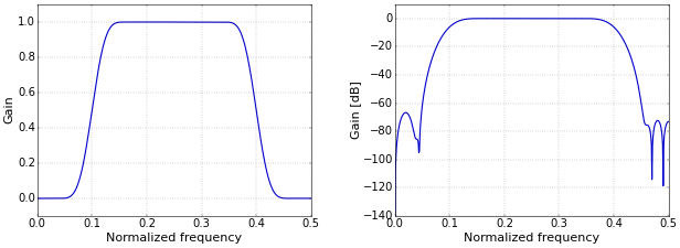
Hence, a band-pass filter can be created from a low-pass and a high-pass filter with appropriate cutoff frequencies by convolving the two filters. The example band-pass filter of Figure 1 has fL=0.1 and fH=0.4, with b=0.08 as in the articles on low-pass and high-pass filters.
 Figure 1. Band-pass filter frequency response on a linear (left) and logarithmic (right) scale.
Band-Reject Filter
A band-reject filter rejects frequencies between the lower limit fL and the higher limit fH, and passes other frequencies. As for the band-pass filter, you can get this result in two steps. In the first step, you apply a low-pass filter with cutoff frequency fL,
xlpf,L[n]=x[n]∗hlpf,L[n],
where x[n] is the original signal, hlpf,L[n] is the low-pass filter with cutoff frequency fL, and xlpf,L[n] is the low-pass-filtered signal.
The result is a signal in which the frequencies in the rejection interval have been eliminated, but in which the frequencies higher than fH are also gone. This can be corrected by filtering the original signal again, with a high-pass filter with cutoff frequency fH, and adding the result to the first signal,
xbr,LH[n]=xlpf,L+x[n]∗hhpf,H[n],
where hhpf,H[n] is the high-pass filter with cutoff frequency fH, and xbr,LH[n] is the required band-reject-filtered signal.
You can again to better and combine both operations into a single filter. You can write
xbr,LH[n]=x[n]∗hlpf,L[n]+x[n]∗hhpf,H[n]=x[n]∗(hlpf,L[n]+hhpf,H[n]),
where the last step follows from the distributive property of convolution. This means that the required band-reject filter is
hbr,LH[n]=hlpf,L[n]+hhpf,H[n].
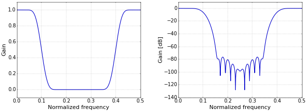
Hence, a band-reject filter can be created from a low-pass and a high-pass filter with appropriate cutoff frequencies by adding the two filters. The example band-reject filter of Figure 2 has fL=0.1 and fH=0.4, with again b=0.08.
 Figure 2. Band-reject filter frequency response on a linear (left) and logarithmic (right) scale.
Python Code
In Python, all these formulas can be implemented concisely. The first code fragment shows how to implement a band-pass filter.
from __future__ import division

import numpy as np

fL = 0.1  # Cutoff frequency as a fraction of the sampling rate (in (0, 0.5)).
fH = 0.4  # Cutoff frequency as a fraction of the sampling rate (in (0, 0.5)).
b = 0.08  # Transition band, as a fraction of the sampling rate (in (0, 0.5)).
N = int(np.ceil((4 / b)))
if not N % 2: N += 1  # Make sure that N is odd.
n = np.arange(N)

# Compute a low-pass filter with cutoff frequency fH.
hlpf = np.sinc(2 * fH * (n - (N - 1) / 2))
hlpf *= np.blackman(N)
hlpf = hlpf / np.sum(hlpf)

# Compute a high-pass filter with cutoff frequency fL.
hhpf = np.sinc(2 * fL * (n - (N - 1) / 2))
hhpf *= np.blackman(N)
hhpf = hhpf / np.sum(hhpf)
hhpf = -hhpf
hhpf[(N - 1) // 2] += 1

# Convolve both filters.
h = np.convolve(hlpf, hhpf)
The second code fragment shows how to implement a band-reject filter.
from __future__ import division

import numpy as np

fL = 0.1  # Cutoff frequency as a fraction of the sampling rate (in (0, 0.5)).
fH = 0.4  # Cutoff frequency as a fraction of the sampling rate (in (0, 0.5)).
b = 0.08  # Transition band, as a fraction of the sampling rate (in (0, 0.5)).
N = int(np.ceil((4 / b)))
if not N % 2: N += 1  # Make sure that N is odd.
n = np.arange(N)

# Compute a low-pass filter with cutoff frequency fL.
hlpf = np.sinc(2 * fL * (n - (N - 1) / 2))
hlpf *= np.blackman(N)
hlpf /= np.sum(hlpf)

# Compute a high-pass filter with cutoff frequency fH.
hhpf = np.sinc(2 * fH * (n - (N - 1) / 2))
hhpf *= np.blackman(N)
hhpf /= np.sum(hhpf)
hhpf = -hhpf
hhpf[(N - 1) // 2] += 1

# Add both filters.
h = hlpf + hhpf
Applying the filter h to a signal s is done by convolution, as for the low-pass and high-pass filters, and can again be as simple as writing the single line:
s = np.convolve(s, h)
Filter Design Tool
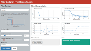
This article is complemented with a Filter Design tool. Experiment with different values for fL and fH, visualize the resulting filters, and download the filter coefficients. Try it now!

# Add both filters.
h = hlpf + hhpf
This line:
h = hlpf + hhpf
should be changed to:
h = np.convolve(hlpf, hhpf)
No, the code as given is correct. Note that the the filters are combined in a different way for band-pass and band-reject. The mathematical reasoning behind this is given in the body of the article.
Thanks so much for this tutorial! Its very helpful. One quick comment:
Based on running this code, it seems like there could be a slight correction
hhpf[(N - 1) // 2] += 1should be
hhpf[(N - 1) // 2 + 1] += 1Thanks for your kind words! I think the code is correct as I wrote it. Let's look at an example: I make sure that
Nis odd, for example,N=5. This means that the coefficients are numbered 0, 1, 2, 3, 4.(N-1)//2equals two, so I indeed add one to the middle coefficient.Hi Tom,
Thanks for the article. It's very much helpful:)
But the results(I mean Filter Plots), I got, are pretty much different as shown above with same Cutoff Frequency.
Thanks again:)
Could you please give me the code on how to plot the above plots
I have a post on that: How to Plot the Frequency Response of a Filter.
Hi Tom
Thanks for the article! Could you also implement a band pass filter by subtracting two low pass filters with cutoffs fH and fL?
Hi Marcello,
Yes, that is indeed also a possibility. And it even results in a shorter filter... The approach that I describe above is the most used one, I think, probably because it follows directly from the procedure of removing the low and the high frequencies in two steps. I'm considering writing a short new blog post about this, as I've done for the alternative approach to compute a high-pass filter in Spectral Reversal to Create a High-Pass Filter. Thanks for the hint!
Hi Tom,
Everything on your blog is extremely helpful, especially for someone who only has a basic grasp of signal processing. Your explanations are great and the filter design tool is a home run. It's great to be able to see how changes in parameters impact filter design with a click of the mouse.
Here's the issue. I've noticed your filter design tool calculates everything based on regular or linear frequency (f) which is measured in cycles per second or hertz. My filter work is all based on angular frequency (w) which is measured in radians per year. To use your filter design tool would I have to convert f to w by using w=2(pi)f? Would that even work given the dramatic difference in time sampling? How difficult would it be to add a drop-down box that includes angular frequency in different time increments?
Thanks!
Curt
Hi Curt,
I'm not entirely sure that I understand what you mean, but I think that your main issue with the tool is that the frequency cannot be set to something smaller than 1 Hz, which is what you'd need for things measured in days or years. This would not necessarily be hard to adapt, but I'm not sure that I'll find the time…
However, I think that you can use normalized frequency (which is what you get with the sampling rate set to 1 Hz, the default) to do what you want. The normalized frequency is relative to the sampling rate in Hz.
To give an example: Say that you sample something once an hour (which would make the sampling rate 1/3600 Hz). This implies that the 0.5 on the frequency scale corresponds with things that occur once every 2 hours (1/7200 Hz). And say that you want to create a low-pass filter to get rid of everything that changes more often than daily. A day is 24 hours, and 2 is 1/12th of that, so the cutoff frequency in the tool must be set to 0.5/12=0.04167 Hz to achieve that.
I hope this helps!
Tom
This is very helpful. Thanks Tom!
Add new comment