When researching what to include in The Moving Average as a Filter and Variations on the Moving Average, I came across a lot of references to applications in the financial sector. This is not my forte, but, just for fun, I gave a few of the moving averages that are used there the same treatment as the filters in Variations on the Moving Average.
For completeness, I first repeat the basic moving average (Figure 1), again with three extra samples on both sides that are not part of the impulse and step responses, for clarity.
 Figure 1. Impulse (left), step (middle), and frequency (right) responses for the moving-average.
Weighted Moving Average (WMA)
A typical usage of the weighted moving average (WMA) is the technical analysis of stocks. The basic moving average is also used there, but the WMA gives (much) more importance to the most recent prices. The accepted definition of the WMA seems to be linearly decreasing weights (Figure 2). For \(N\) points, the highest weight is \(N\) and the lowest weight is \(1\). These weights are then divided by the sum of all coefficients to normalize them.
 Figure 2. Impulse (left), step (middle), and frequency (right) responses for the WMA.
This filter is not linear phase, since it is not symmetrical.
Exponentially Weighted Moving Average (EWMA)
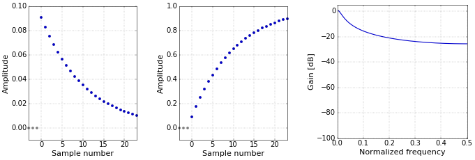
Still for the technical analysis of stocks, the exponentially weighted moving average (EWMA) is sometimes used instead of the WMA, to put even more emphasis on the most recent prices. The EWMA is often simply called the exponential moving average (EMA). The common definition of the EWMA seems to coincide exactly with the definition of a low-pass single-pole IIR filter. See that article for details. In that article, I use a parameter \(d\) as the decay of the single-pole filter. The EWMA typically uses a parameter \(\alpha=1-d\). Furthermore, there seems to be some sort of consensus to compute the value of \(\alpha\), for an average of “length” \(N\), as \(\alpha=1/(N+1)\). An example for \(N=21\) is shown in Figure 3.
 Figure 3. Impulse (left), step (middle), and frequency (right) responses for the EWMA.
This filter is also not linear phase. Note that the impulse response is infinite, and that the figure only shows the first 24 samples. The frequency response was computed on the full impulse response, or at least on a much longer version, not on those first 24 samples (if you do that, you get the same kind of “wobbles” as in Figure 2).
Spencer’s 15-Point Moving Average
A more specialized filter is Spencer’s 15-point moving average (Figure 4). I admit that I don’t really know what it’s used for… The definition of this filter is given by an explicit list of coefficients: −3, −6, −5, 3, 21, 46, 67, 74, 67, 46, 21, 3, −5, −6, −3, again normalized in the plot.
 Figure 4. Impulse (left), step (middle), and frequency (right) responses for Spencer’s 15-point moving average.
This filter is linear phase, since it is symmetrical.
If you are in the financial sector and use these things, let me know in the comments whether you need me to dig further into this stuff from a signal processing point of view.
Digital filters for financial work need to have zero (or near zero) lag. This translates into zero-phase response. However all zero phase filters that I know of are non-causal. Find a causal zero-phase lowpass filter, and we could rule the world!
btw, John Ehlers is the man for using DSP in finance. Do look up his work!
Hi Mark, AFAIK if you have previously sampled offline data in a computer file rather than live data you a receiving from an ADC in real-time you can use a zero phase non-causal filters without any issues.
This is one of those commonly misunderstood things that is not discussed properly in the literature which typically assumes (implicitly) real-time applications of DSP in all discussions.
Add new comment