How to Create a Simple High-Pass Filter

Summary: This article shows how to create a simple high-pass filter, starting from a cutoff frequency \(f_c\) and a transition bandwidth \(b\). This article is complemented by a Filter Design tool that allows you to create your own custom versions of the example filter that is shown below, and download the resulting filter coefficients.

In contrast to what you might expect, the procedure to create a simple high-pass filter is not a variation on the procedure to create a low-pass filter that I explained in How to Create a Simple Low-Pass Filter. The high-pass filter is created by building a low-pass filter first, and then using spectral inversion to convert it into a high-pass one. An alternative for spectral inversion is spectral reversal, as described in Spectral Reversal to Create a High-Pass Filter.

The windowed-sinc filter that is described in this article is an example of a Finite Impulse Response (FIR) filter.

Spectral Inversion

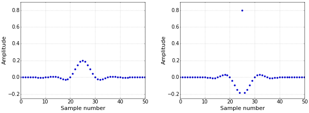
Starting from the cutoff frequency \(f_c\) and the transition bandwidth (or roll-off) \(b\), first create a low-pass filter as described in How to Create a Simple Low-Pass Filter. The normalized low-pass filter from that article, again for \(f_c=0.1\) and \(b=0.08\), is shown as the left image in Figure 1.

The spectral inversion of a filter \(h[n]\) is defined as follows.

1. Change the sign of each value in \(h[n]\).
2. Add one to the value in the center.

This produces the filter shown as the right image in Figure 1.

Figure 1. Low-pass (left) and high-pass (right) filters.

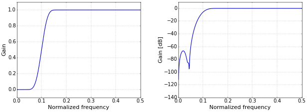
For this procedure to work, the low-pass filter must have left-right symmetry, but the filters from the mentioned article do have this property. The frequency response of the high-pass filter is then as shown in Figure 2.

Figure 2. Frequency response on a linear (left) and logarithmic (right) scale.

This frequency response is an “upside down” version (look at the linear representation for this) of the frequency response of the low-pass filter. This implies that designing a high-pass filter in this manner is exactly as straightforward as designing a low-pass one.

Why Does Spectral Inversion Work?

Spectral inversion is based on the following idea. A low-pass filter generates a signal with the high frequencies removed. Hence, if you subtract this signal from the original one, you have exactly the high frequencies. This means that you can implement a high-pass filter in two steps. First, you compute

\[x_\mathrm{lpf}[n]=x[n]*h_\mathrm{lpf}[n],\]

where \(x[n]\) is the original signal, \(h_\mathrm{lpf}[n]\) is the low-pass filter, and \(x_\mathrm{lpf}[n]\) is the low-pass-filtered signal. The asterisk represents convolution. Second, you compute

\[x_\mathrm{hpf}[n]=x[n]-x_\mathrm{lpf}[n],\]

where \(x_\mathrm{hpf}[n]\) is the high-pass-filtered signal.

The alternative is to adapt the filter through spectral inversion. To show that spectral inversion has exactly the same result, first note that \(x[n]=x[n]*\delta[n]\), where \(\delta[n]\) is a simple impulse, as defined in Impulse Response. You can then write

\[x_\mathrm{hpf}[n]=x[n]-x_\mathrm{lpf}[n]=x[n]*\delta[n]-x[n]*h_\mathrm{lpf}[n]=x[n]*(\delta[n]-h_\mathrm{lpf}[n]),\]

where the last step follows from the distributive property of convolution. This means that the required high-pass filter is

\[h_\mathrm{hpf}[n]=\delta[n]-h_\mathrm{lpf}[n],\]

which is exactly the procedure that I’ve described before.

Python Code

In Python, this can again be implemented concisely (of course, the asterisk in the Python code performs multiplication, not convolution).

from __future__ import division
 
import numpy as np
 
fc = 0.1  # Cutoff frequency as a fraction of the sampling rate (in (0, 0.5)).
b = 0.08  # Transition band, as a fraction of the sampling rate (in (0, 0.5)).
N = int(np.ceil((4 / b)))
if not N % 2: N += 1  # Make sure that N is odd.
n = np.arange(N)
 
# Compute a low-pass filter.
h = np.sinc(2 * fc * (n - (N - 1) / 2))
w = np.blackman(N)
h = h * w
h = h / np.sum(h)
 
# Create a high-pass filter from the low-pass filter through spectral inversion.
h = -h
h[(N - 1) // 2] += 1

Applying the filter \(h\) to a signal \(s\) is done by convolution, as for the low-pass filter, and can again be as simple as writing the single line:

s = np.convolve(s, h)

As an application of this, I combine low-pass and high-pass filters in How to Create Simple Band-Pass and Band-Reject Filters.

Filter Design Tool

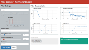
This article is complemented with a Filter Design tool. Experiment with different values for \(f_c\) and \(b\), visualize the resulting filters, and download the filter coefficients. Try it now!

Filter designer.