How to Create a Configurable Filter Using a Kaiser Window

This article explains how to create a windowed-sinc filter with a Kaiser (or Kaiser-Bessel) window. The windowed-sinc filters in previous articles such as How to Create a Simple Low-Pass Filter typically had two parameters, the cutoff frequency \(f_c\) and the transition bandwidth (or rolloff) \(b\). With a Kaiser window, there is a third input parameter \(\delta\), the ripple. All three parameters are illustrated in Figure 1.

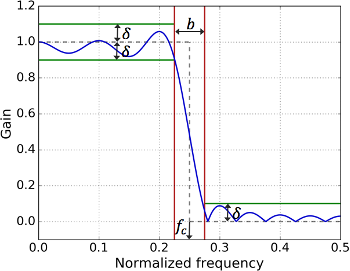Figure 1. Parameters of a low-pass filter with a Kaiser window.

For the specific case of the Kaiser window, the same \(\delta\) is used in the passband and in the stopband. The impulse response of the underlying sinc filter is, as in How to Create a Simple Low-Pass Filter, still defined as

\[h[n]=2f_c\mathrm{sinc}(2f_cn),\]

where \(f_c\) is the cutoff frequency, and where \(n\) runs from \(-\infty\) to \(+\infty\). Remember that this range of \(n\) is actually the reason that a window is necessary. The impulse response of the ideal filter is infinite, and needs to be “shortened” in a way that is better than simple truncation.

The main advantage of the Kaiser window is that it is more configurable than, e.g., the Blackman window. The acceptable ripple of the filter can be specified, while it is fixed (but known) for the basic window types.

Kaiser Window

The definition of the Kaiser window is given by

\[w[n]=\frac{I_0\left(\beta\sqrt{1-\left(\frac{2n}{N-1}-1\right)^2}\right)}{I_0(\beta)},\]

with \(N\) the length of the filter, \(n\) running from zero to \(N-1\), and \(\beta\) a parameter that can be chosen freely (see below). \(I_0(\cdot)\) is the zeroth-order modified Bessel function of the first kind. Especially with the Bessel function, this expression looks more complicated than the expressions for windows such as Blackman. However, Bessel functions have many applications and are directly available in Python and MATLAB.

By varying the length \(N\) and the parameter \(\beta\), the properties of the final filter, which is the product of \(h[n]\) (shifted to the range \([0,N-1]\)) and \(w[n]\), can be determined. This results in the three mentioned tunable parameters, the cutoff frequency \(f_c\), the transition bandwidth \(b\), and the ripple \(\delta\). Traditionally, \(\delta\) is seen as the tunable parameter, and a new parameter \(A\) is then computed as

\[A=-20\log_{10}(\delta).\]

Personally, I would suggest that you take this \(A\) to be the tunable parameter, since it is simply the attenuation of the filter in the stopband in dB. If the ripple in the passband is very important, you might not be able to do that. However, for a typical filter that is used to remove a range of frequencies more or less completely, you’ll need to make \(A\) relatively large, resulting in a small ripple in the passband anyway.

Kaiser then empirically, through numerical experimentation, determined which value of \(\beta\) to use to end up with a given value for \(A\), as

\[\beta=\begin{cases}
0.1102(A-8.7),&A\gt 50\\[0.3em]
0.5842(A-21)^{0.4}+0.07886(A-21),&21\leq A\leq 50\\[0.3em]
0,&A\lt 21
\end{cases}.\]

The final parameter that you need is then the filter length \(N\), also determined empirically by Kaiser as

\[N=\dfrac{A-8}{2.285\cdot2\pi b}+1.\]

I’ve added the term \(+1\) because the formula of Kaiser estimates the filter order, which is one less than the filter length. Additionally, you often still want the filter to have an odd length, so that its delay is an integer number of samples, so you might have to do another \(+1\) if the original estimate is even…

And that’s it. You can then use these parameters \(\beta\) and \(N\) in the expression for \(w[n]\) above to create a Kaiser window with the given transition bandwidth \(b\) and attenuation in the stopband \(A\).

Examples

For the parameters \(f_c=0.25\), \(b=0.1\), and \(A=40\), the result is given in Figure 2. In this case, \(N=25\) and \(\beta=3.395\).

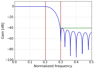Figure 2. Frequency response of a low-pass filter with a Kaiser window; A=40.

For the parameters \(f_c=0.125\), \(b=0.05\), and \(A=60\), the result is given in Figure 3. In this case, \(N=75\) and \(\beta=5.653\).

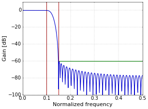Figure 3. Frequency response of a low-pass filter with a Kaiser window; A=60.

To create other types of filters such as high-pass or band-pass, the standard techniques can be used, for example as described in How to Create a Simple High-Pass Filter and How to Create Simple Band-Pass and Band-Reject Filters. Figure 4 shows an example of a high-pass filter that was created through the technique described in Spectral Reversal to Create a High-Pass Filter, from the same parameters that were used for Figure 3.

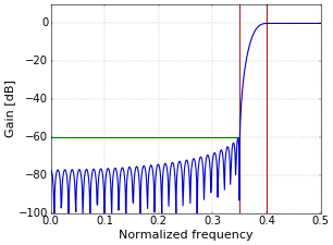Figure 4. Frequency response of a high-pass filter with a Kaiser window; A=60.

Python Code

In Python, all these formulas can be implemented concisely.

from __future__ import division
 
import numpy as np
 
fc = 0.25  # Cutoff frequency as a fraction of the sampling rate (in (0, 0.5)).
b = 0.1    # Transition band, as a fraction of the sampling rate (in (0, 0.5)).
A = 40     # Attenuation in the stopband [dB].
 
N = int(np.ceil((A - 8) / (2.285 * 2 * np.pi * b))) + 1
if not N % 2: N += 1  # Make sure that N is odd.
if A > 50:
    beta = 0.1102 * (A - 8.7)
elif A <= 50 and A >= 21:
    beta = 0.5842 * (A - 21) ** 0.4 + 0.07886 * (A - 21)
else:
    beta = 0
n = np.arange(N)
 
# Compute sinc filter.
h = np.sinc(2 * fc * (n - (N - 1) / 2))
 
# Compute Kaiser window.
w = np.i0(beta * np.sqrt(1 - (2 * n / (N - 1) - 1) ** 2)) / np.i0(beta)
 
# Multiply sinc filter by window.
h = h * w
 
# Normalize to get unity gain.
h = h / np.sum(h)

Applying the filter \(h\) to a signal \(s\) by convolving both sequences can then be as simple as writing the single line:

s = np.convolve(s, h)

In the Python script above, I compute everything in full to show you exactly what happens, but, in practice, shortcuts are available. For example, the Kaiser window can be computed with w = np.kaiser(N, beta).

Filter Design Tool

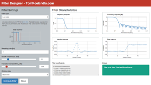
This article is complemented with a Filter Design tool. With respect to Kaiser windows, it allows building low-pass, high-pass, band-pass, and band-reject filters. Try it now!

Filter designer.